I – Background Information
The ever-increasing population in cities across the world increases the pressure and expectation of the availability and punctuality of public transport services. Thus, consequences associated with unexpected incidents, involving transport assets, include high repair costs and major disruptions to the entire transport network, ultimately having a detrimental effect on the business. The identification and implementation of an appropriate maintenance strategy can help in the optimization of maintenance planning and scheduling, decrease rolling stock downtime, and increase the life expectancy of assets such as trams.
The main maintenance strategies today rely mostly on preventive maintenance as well as on condition maintenance, however, although still relevant, preventive maintenance typically results in over maintaining assets and high cost. It is subsequently of high interest to increase the use of advanced maintenance strategies and reduce reactive maintenance events. Thus, allowing more time to respond which in turn enables greater flexibility to dynamically plan an appropriate maintenance strategy and decrease cost.
The goal of this project was to provide precise and reliable predictions to optimize planning and downtime maintenance of trams using data from a wheel measurement device.
II – Data Pre-processing
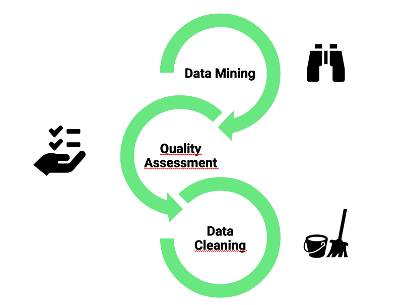
The first task in any data science project consists of transforming raw data into a more understandable format. To better understand the state of the data, and to determine the information that is usable, a quality assessment is first conducted.
The quality assessment enables us to identify missing values/measurements, corrupted values, incoherent values, and duplicate values.
This quality assessment is followed by a data cleaning process to remove the flawed measurements/values. In this project, we removed over 50% of the data at hand due to missing and incoherent values. Furthermore, duplicates were removed along with outliers. For the removal of outliers, we used the Z-score metric, where we calculate the Z-score for every single target value (the measurement we want to predict) and remove the values for which the z-score is above a certain threshold.
The Z-score, also known as the standard score, measures the number of standard deviations an element is from the population mean. The Z-score is negative if a given element is below the mean, and positive if it is above the mean. Logically the closer the Z-score to zero, the closer a given element is to the mean of the population. In this project, the Z-score is calculated to determine which measurements for a unique tram wheel are outliers and need to be rejected from the data set. Subsamples for each unique tram wheel are created to calculate the Z-score for the given measurements and a carefully fixed threshold allows us to reject any observation that differs greatly from the population mean.
Lastly, part of the of the preprocessing task is to integrate metadata, from different sources, that may help us understand the behavior of the data we initially have. When integrating data from multiple sources it Is of high importance to define a schema, which all data must respect, in order to maintain consistency and compatibility.
III – Data Exploration/Analysis
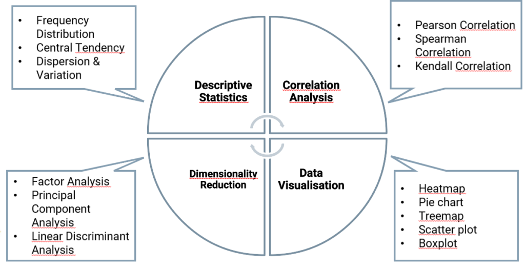
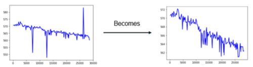
Once the preprocessing step is complete, the next step is to explore the data using visualization tools, and summarizing functions.
For example, we could visualize the trends in wheel measurements over time along with various weather measurements.
In addition, we calculated summary statistics such as the median, average, standard deviation of the variables in the data set, as well as the average wheel deterioration pre-covid19 lockdown restrictions and during covid19 lockdown restrictions imposed throughout Europe. Knowing some trams serviced at the same rate during the lockdown compared to pre-lockdown, we took advantage of this unprecedented period to investigate the effect the passenger load has on the deterioration of the wheels.
Another step to better understand the data, is to understand the relationship between the variables we possess. Specifically, the relationship between the target variable and the remaining variables in the dataset. There exists several different correlation statistics, such as the Pearson correlation, the Kendall correlation, Spearman correlations, each having their own perks. In this project, we decided to use the Pearson correlation, as we look to measure the relationship between the wheel measurement variable and subsequent linearly related variables.
As a side note, the Pearson correlation coefficient yields values between -1 and 1, meaning the closer the coefficient is to -/+1 the higher the degree of association between the two variables. On the other hand, a coefficient equal to 0 indicates no relationship between the two variables.
Furthermore, correlation coefficients enable us to reduce the number of input variables, by selecting the variables with the strongest relationship with the target variable and are believed to be most useful when developing a predictive model. As we reduce the number of variables used to predict the target variable, we also reduce the computational cost of the model.
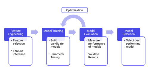
IV – Model Build :
Train test split:
Since we are dealing with time series data, any random sampling approach, to select instances from the population to compute the expected performance, should be avoided. These approaches assume that the instances, in this case the measurements, are independent. However, the wheel measurements at a time t are highly dependent on the previous measurements at time t − 1. Applying a random sampling approach to evaluate our model would overestimate the performance of the model and lead us to a false confidence state. This problem is solved by creating subsets of the data to generate training and validation sets. The training set therefore contains 80% of data, according to the timestamp of the measurements, and the validation set contains the remaining 20%.
Evaluation method:
In such a practical application as this project, it is fundamental that the results are accurately evaluated. As the goal is to forecast the wear and tear of rolling stock assets, which ultimately leads to maintenance planning, the performance of the predictions must be measured in an effective manner. This is paramount in avoiding maintenance shortfall or unnecessary maintenance, which could in turn lead to higher costs. Furthermore, it is paramount to determine a suitable evaluation metric for the given problem. As we are dealing with a regression task, we want to measure the differences between the predicted values and the observed values. For this purpose, &. The RMSE corresponds to the quadratic mean of the differences between the observed values and the predicted values.
V- Results :
Ablation study:
To understand the behavior of the predictive model, and the importance of certain features, an ablation study was conducted. An ablation study consists of removing a feature from the model to access the effect it has on the performance. By removing certain features one by one, we’re able to understand the importance they have in the construction of the predictive model, and to identify which features could ultimately be left out.
SHAP values:
Another way of discovering which features are the most important for the predictive model is to calculate the SHAP values. SHAP, Shapley Additive Explanations, is a method proposed by S.M.Lundberg and Su-In Lee for interpreting the predictions of complex models. This method attributes the change in the expected prediction to each feature when conditioning on the latter.
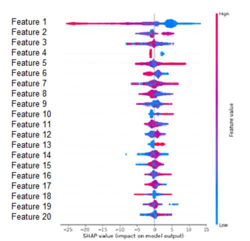
The Figure below orders the features according to the sum of the SHAP value over all samples in the training set. This Figure shows the impact that the features have on the model output depending on the feature value. For example, a high value of ‘Feature 1’ lowers the predicted value. On the other hand, a high value of ‘Feature 13’ increases the predicted value.
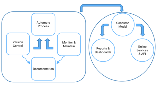
VI – Conclusion :
The main benefits of predictive maintenance improve the overall day to day operations, especially in a fast-paced environment such as public transport. In the current context, the fruition of this project would enable the maintenance teams to integrate planning into a single platform. On one hand allowing them to visualize and interpret real time data, on a day to day operational actions, and on the other hand providing them with maintenance decision making based on state-of-the-art asset predictions. The development of such a platform yields the possibility for maintenance teams to visualize the predicted and forecasted deterioration and failures of assets and, suggest to users the correct course of action to take.
More generally and in a larger context, as cities across the world rely deeply on public transport, reliability is at the forefront of transportation strategies. It is therefore of upmost importance that asset management is optimized through predictive maintenance. Through future predictions, transportation services can ensure maintenance is performed only when required before imminent failure, thus reducing unnecessary downtime of assets and costs associated with over-maintaining equipment. Preventing such failures limits the severity of damages to the assets and improves the life expectancy of equipment. This ability in turn provides optimal planning and storing for spare parts, rather than having an overabundance of stock. Lastly, predictive maintenance offers the opportunity to greatly reduce the number of incidents on the transport network, which in turn improves the all-important passenger safety and comfort.
 Written by Magnus Kinder, Data Scientist @ Valkuren